Inside the Cortex: turning an AI's memory into a 3D star map

Start here: a galaxy made of thoughts

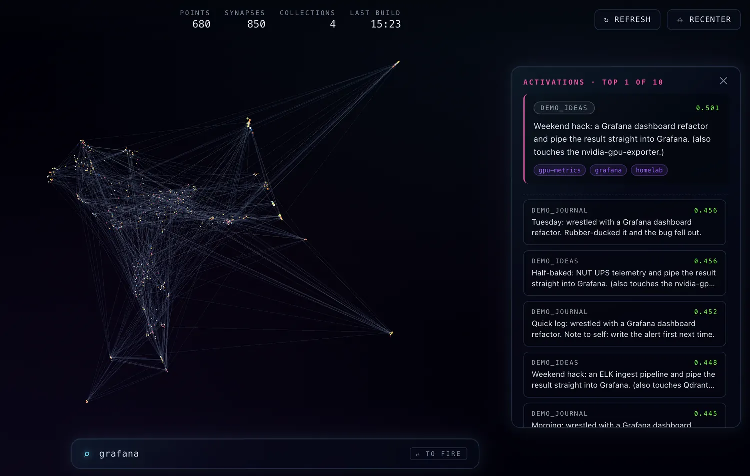
Open the demo — cortex-demo.akciali.com — and you are looking at a cloud of glowing points drifting in 3D. You can grab it, spin it, fly into it. Each point is a single memory: one note, one fact, one decision. Thin threads run between some of them — those are links, thoughts that reference one another. A few points pulse brighter than the rest: those are the recent memories, the things learned in the last day.

That’s the whole idea in one sentence: I took the memory of an AI assistant and drew it as a star field you can explore.

You don’t need to know anything about machine learning to enjoy it. Colour tells you age — the youngest memories burn blue-white like hot young stars, the oldest fade to deep red, exactly the way real stars are classified by temperature. Distance tells you meaning — memories about the same topic naturally clump together, while unrelated ones drift apart. Fly toward a cluster and you’ll find a neighbourhood of related ideas; the empty space between clusters is where the subject changes.

So far, so pretty. But how does a computer decide that two notes are “about the same thing” and should sit next to each other? That’s where it gets interesting.

What is actually stored

Behind the visualization is a vector database. When the assistant wants to remember something — “the backup job keeps eight copies”, “Friday’s deploy went green” — it doesn’t store the sentence as text for searching. It stores a list of numbers called an embedding.

An embedding is produced by a small neural network (here, a model called embeddinggemma, run locally through Ollama). You feed it a piece of text and it hands back a fixed-length list of numbers — 768 of them in this case. The magic property is this: texts that mean similar things get similar lists of numbers. “The pump runs at 50%” and “AIO pump set to half speed” land close together; “I love my kids” lands somewhere completely different.

You can think of each memory as having an address in a 768-dimensional space. Meaning becomes geometry: similarity is just distance. That’s what makes the whole thing searchable, and it’s what makes the clusters in the visualization real rather than decorative.

The catch: you can’t see 768 dimensions

A space with 768 axes is perfectly comfortable for a computer and completely impossible for a human eye. We get three dimensions, maybe four if you count time. So to draw the memory, we need to squash 768 dimensions down to 3 — without destroying the structure that makes it meaningful.

That’s a classic problem called dimensionality reduction, and the tool here is UMAP (Uniform Manifold Approximation and Projection). UMAP’s job is to find a 3D arrangement of the points where things that were neighbours in 768D are still neighbours in 3D. It doesn’t care about preserving exact distances across the whole map — it cares about keeping local neighbourhoods intact. Two knobs matter most:

• n_neighbors — how much local vs. global structure to respect. Small values draw tight, fragmented islands; larger values give a smoother, more connected cloud.
• min_dist — how tightly points are allowed to pack. Small values let clusters condense into dense knots; larger values spread them out.

Run UMAP on every memory’s 768-number address, and out come three numbers per memory: x, y, z. Now they can be stars.

From numbers to a night sky

The browser side is a Three.js scene. Each memory becomes an instanced sprite placed at its (x, y, z). Three layers of meaning are painted on top of the raw geometry:

• Colour by age. Every memory carries a timestamp. The renderer maps age onto a stellar O-B-A-F-G-K-M palette — the real spectral sequence astronomers use — stretched across the actual age range of the dataset, so the map always uses its full colour range whether your memories span a week or two years.
• Synapses. When one memory explicitly references another, a faint line is drawn between them. Most stay a quiet grey-blue so the structure reads without shouting; links that touch a very recent memory keep their stellar colour, so you can see where new thinking is wiring itself into the old.
• Highlight. Memories from the last 24 hours pulse gently. It’s the same instinct as a “what’s new” badge, except it’s spatial — you can watch where recent activity lights up the map.

There’s a subtle data-modelling point here worth calling out: the positions come only from the embeddings, never from the links. UMAP never sees the link graph. So when two clusters end up close, that’s because their content is genuinely related — not because someone drew a line. The links are then layered on top as a second, independent signal. When the two agree, you trust the map more.

Searching the map

Type a query into the demo and something satisfying happens: the matching memories light up wherever they are in the cloud. The mechanism is the same trick as before, run in reverse.

1. Your query text is sent to the same embedding model, producing its own 768-number address.
2. The vector database (Qdrant) finds the stored memories whose addresses are closest — measured by cosine similarity, essentially “do these two arrows point the same way”.
3. The top matches are returned and highlighted.

Because the query and the memories are embedded by the same model, “vector search latency” will surface notes about retrieval performance even if they never use those exact words. You’re searching by meaning, not by keyword.

How the pieces fit together

The moving parts, end to end:

• Ollama serves the embedding model locally, so text never leaves the machine to become a vector.
• Qdrant stores the vectors and answers nearest-neighbour queries.
• A small FastAPI service ties it together: on startup it pulls every vector, runs UMAP once, and caches the 3D projection as a single file so the page loads instantly. It also exposes a search endpoint and a metrics endpoint (scraped by Prometheus/VictoriaMetrics, graphed in Grafana — because of course the memory of the lab is itself monitored).
• A reverse proxy (Caddy) terminates TLS out front.

The instance you’re looking at is a public demo seeded with entirely synthetic data — a few hundred invented notes about lab tooling, generated just to make the cloud look alive. The real memory it’s modelled on lives behind authentication and is never exposed. The privacy boundary isn’t a login bolted onto the demo; it’s that the demo simply has nothing real in it. The engine that draws synthetic notes and the engine that draws real ones are the same code, pointed at different data.

Why bother

A vector database is, normally, the least visual thing imaginable — a table of numbers you query and never look at. Turning it into a place you can walk through changes how you relate to it. You notice when a topic has grown a dense core. You spot the lonely memory with no links and wonder why it never connected. You watch the last day’s thoughts light up at the edges and slowly migrate inward as they age.

It started as a “wouldn’t it be fun” Friday idea. It turns out that giving a memory a shape makes it something you can have intuitions about — and intuitions are exactly what a flat table of 768-dimensional vectors can never give you.

Fly around for a bit: cortex-demo.akciali.com. The blue stars are the new thoughts.